深度学习原理
梯度下降
深度学习简单实现
最基础线性规划实现
1 | import tensorflow as tf |
使用tensorflow的部分接口实现
1 | import tensorflow as tf |
tensorflow高级api使用
所有的深度学习都包含上面几个步骤
- 加载数据
- 迭代
- 梯度更新
- 测试/验证精度计算
因此,tensorflow将上面的固定步骤写在同一的接口中方便使用
1 | import tensorflow as tf |
常见问题
过拟合和欠拟合
过拟合:训练精度很高,测试精度不够(可能)
欠拟合:训练精度不够,测试精度也不够(可能)——模型复杂度不够
过拟合解决
- 更多数据
- 更简单的模型
- 数据增强
Regularization
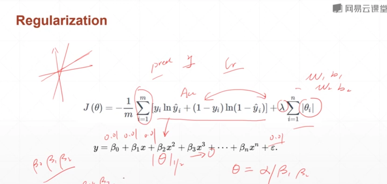
前面是误差,后面是参数的范式,参数的一范式越小说明参数越接近于0,那么拟合出来的模型就越平滑,出现过拟合的可能性就越小
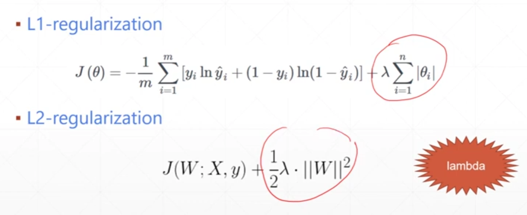
两张regularization方式,分别是一范数二范数
Momentum
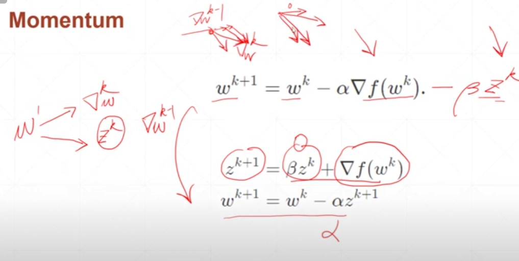
动量设置,参数更改的不仅仅由当前梯度的影像,还与上一次梯度的方向有关
Learning rate
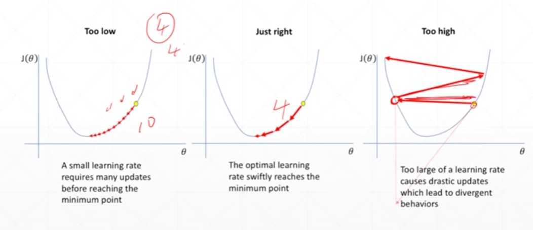
学习率一般刚开始比较大,后续慢慢变小,前期学习率大变化快,后续会较慢
提前取消
如果出现了训练精度还在提高,测试精度不提高了,说明已经过拟合,可以停止训练
Dropout
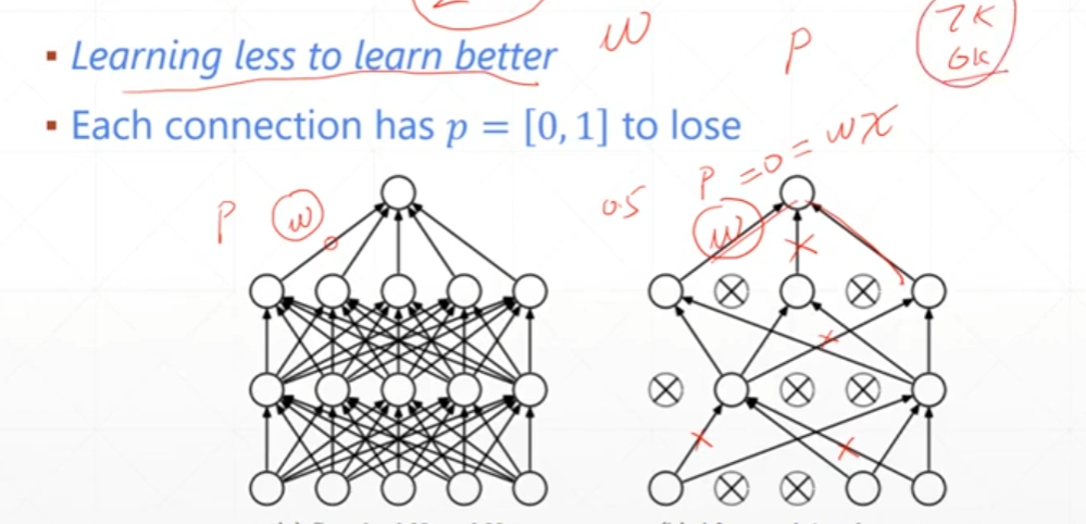
每一次训练都有一些连线可能中断
tensorflow和pytorch的dropout参数是相反的
dropout在做test时不能使用——要手动取消
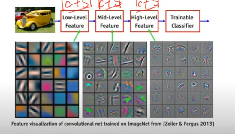
为什么要卷积
为什么要卷积?不使用简单的Dense层?
- 数据存储需求大
视野?滑动窗口?这个窗口是卷积核?cv里面锐化模糊边缘提取的卷积核
卷积核的个数,也就是con2d中的两个参数:
- 卷积核的大小问题
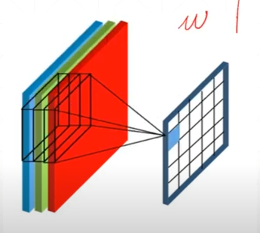
[c, 3, 3]一个卷积核可以将一张图片卷积到一个channels为1的新层次,c为图片的通道数
如图,这个[3, 3, 3]依次对三个通道做乘法,然后将结果加起来得到一个一通道的数据,这个一通道的数据代表着原图像在某一层次上的特征
有时候我们需要更多的特征,这时候就需要[N, c, 3, 3]这样N个卷积来提取特征,就会得到N个通道的特征
如下面的(64, 3)其中的64就是上面的N代表着64个通道的特征,3是卷积核的大小,也就是[c, 3, 3]中的3,c会默认与图片的通道数相同,所以不需要额外设置
1 | conv1 = Conv2D(64, 3, activation='relu', padding='same')(inputs) |
为什么要下采样(池化)
不同的程度可以获取到不同层级的特征